Flow Plots

Flow plots are simply a way of visualizing what LITAP is doing under the hood.

In the following examples, we will be using the output from complete run on the supplied “testELEV.dbf”. You can find the original DEM file in the LITAP extdata folder by using the system.file() function. For more information on the flow_mapper() function see the Getting Started Vignette.

Let’s first copy this file to your working directory with:

file.copy(system.file("extdata", "testELEV.dbf", package = "LITAP"), ".")

## [1] TRUE

library(LITAP)

## LITAP v0.7.0
## LITAP is still in development; Help us by submitting bugs/feature requests: 
## http://github.com/FRDC-SHL/LITAP/issues

# Save output to working directory
flow_mapper("testELEV.dbf", grid = 1, nrow = 90, ncol = 90, clean = TRUE)

## CALCULATING DIRECTIONS

## CALCULATING WATERSHEDS

## REMOVING INITIAL PITS

## CALCULATING POND (GLOBAL) WATERSHEDS

## CALCULATING FILL PATTERNS

## INVERTING DEM

## CALCULATING INVERTED DIRECTIONS

## CALCULATING INVERTED WATERSHEDS

## REMOVING INVERTED PITS

## CREATING REPORT

## Run took: 0.29 min

We will load the rds file (R data files) for the final dems and stats file.

dem <- readRDS("./testELEV/flow/dem_fill.rds")
inverted_dem <- readRDS("./testELEV/flow/dem_inverted.rds")

pond_stats <- readRDS("./testELEV/flow/stats_pond.rds")

Basic maps

By default, the flow_plot() function displays relief maps, using the terrain() and hillShade() functions from the raster package. Note the outer border of dark grey, this represents unknown cells, as the relief calculations do not work on cells without neighbours.

flow_plot(dem)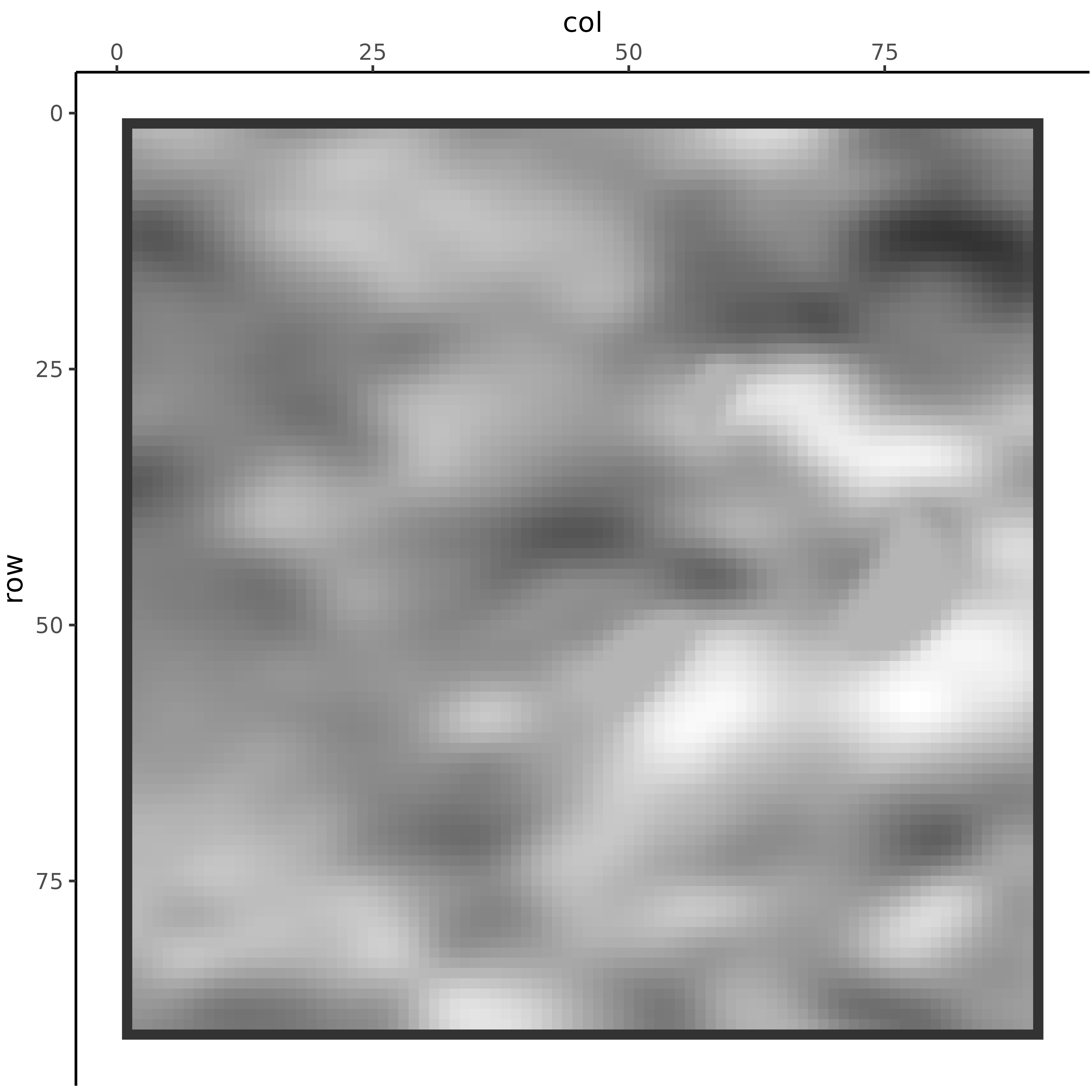

Alternatively, you can plot elevation data directly.

flow_plot(dem, type = "elevation")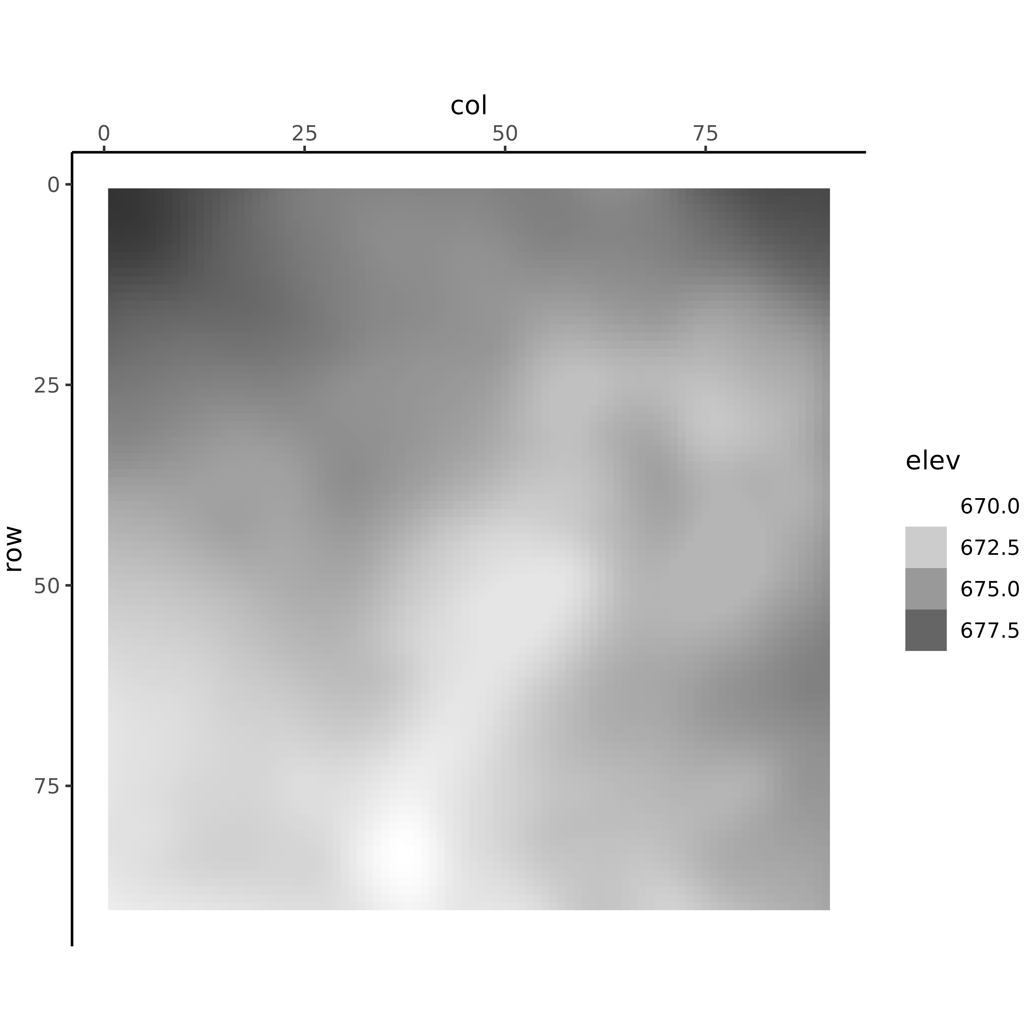

Subsets

You can zoom in on a particular area of interest by specifying row and column limits:

flow_plot(dem, type = "elevation", rlim = c(20, 30), clim = c(35, 45))

Cell numbering

You can number the cells in a plot with seqno = TRUE:

flow_plot(dem, type = "elevation", rlim = c(20, 30), clim = c(35, 45), 
          seqno = TRUE)

If you’re only interested in certain cells, specify which ones with cells = c() and highlight = TRUE

flow_plot(dem, type = "elevation", rlim = c(20, 30), clim = c(35, 45), 
          seqno = TRUE, cells = c(3187:3193, 3336:3343), highlight = TRUE)

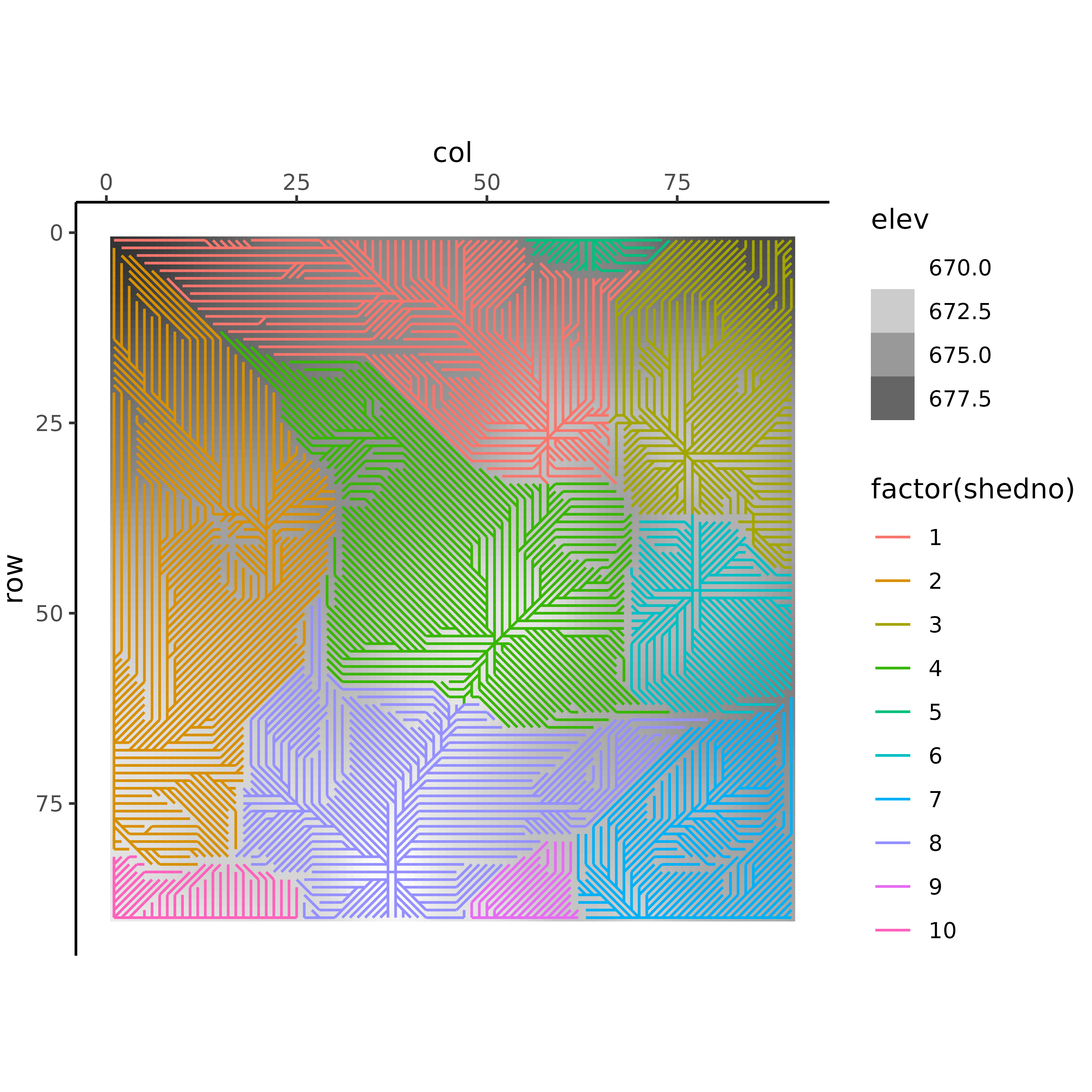
Flow directions

You can plot individual flow directions with dir = TRUE.

flow_plot(dem, type = "elevation", rlim = c(20, 30), clim = c(35, 45), 
          dir = TRUE)

In combination with cell numbers

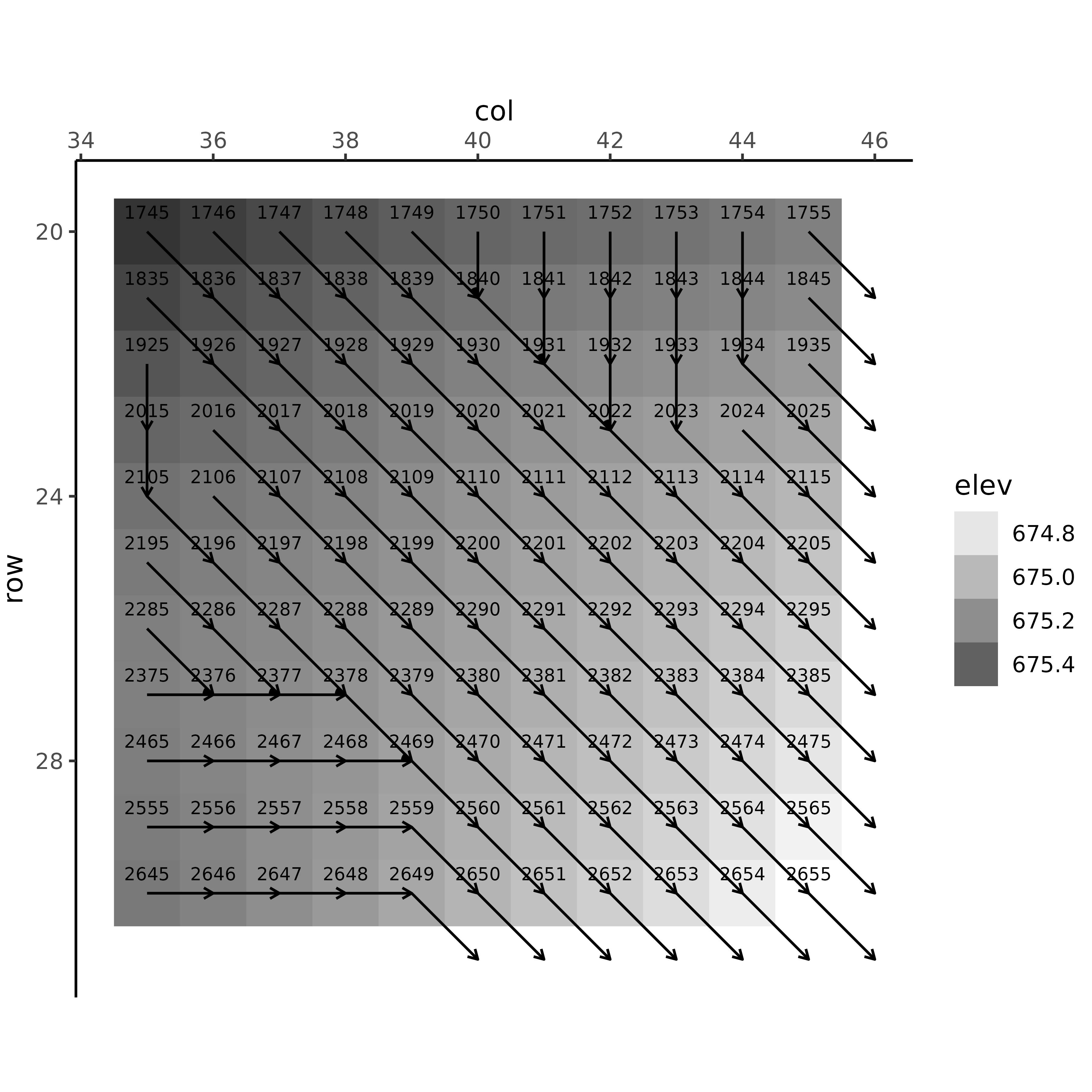
flow_plot(dem, type = "elevation", rlim = c(20, 30), clim = c(35, 45), 
          dir = TRUE, seqno = TRUE)

Only for certain cells (this will show the entire flow path that a given cell is on)

flow_plot(dem, type = "elevation", rlim = c(20, 30), clim = c(35, 45), 
          dir = TRUE, cells = c(3187:3193, 3336:3343))

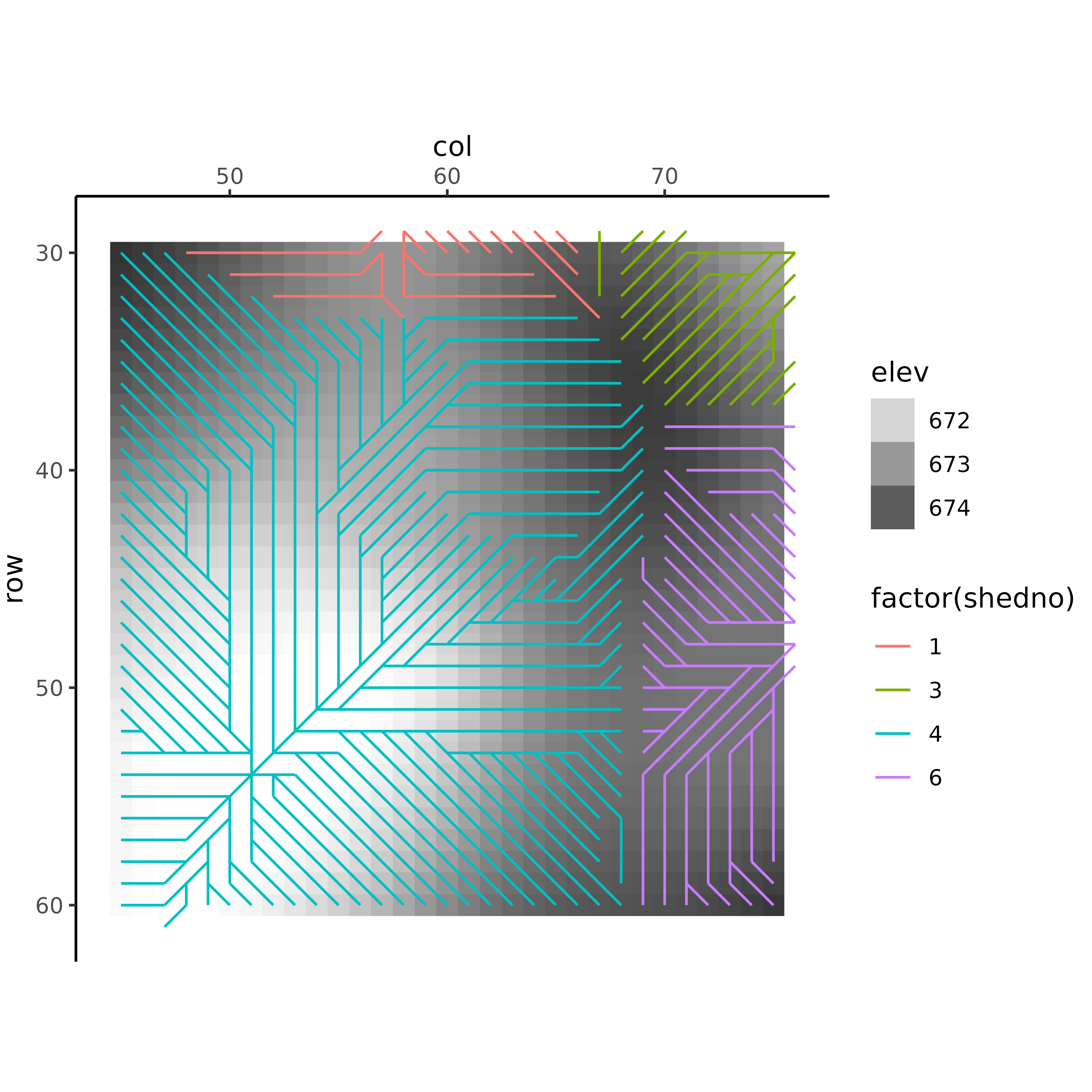
Only for certain cells and show cell numbers

flow_plot(dem, type = "elevation", rlim = c(20, 30), clim = c(35, 45), 
          dir = TRUE, seqno = TRUE, cells = c(3187:3193, 3336:3343))

Highlight the cells of interest

flow_plot(dem, type = "elevation", rlim = c(20, 30), clim = c(35, 45), 
          dir = TRUE, seqno = TRUE, cells = c(3187:3193, 3336:3343), highlight = TRUE)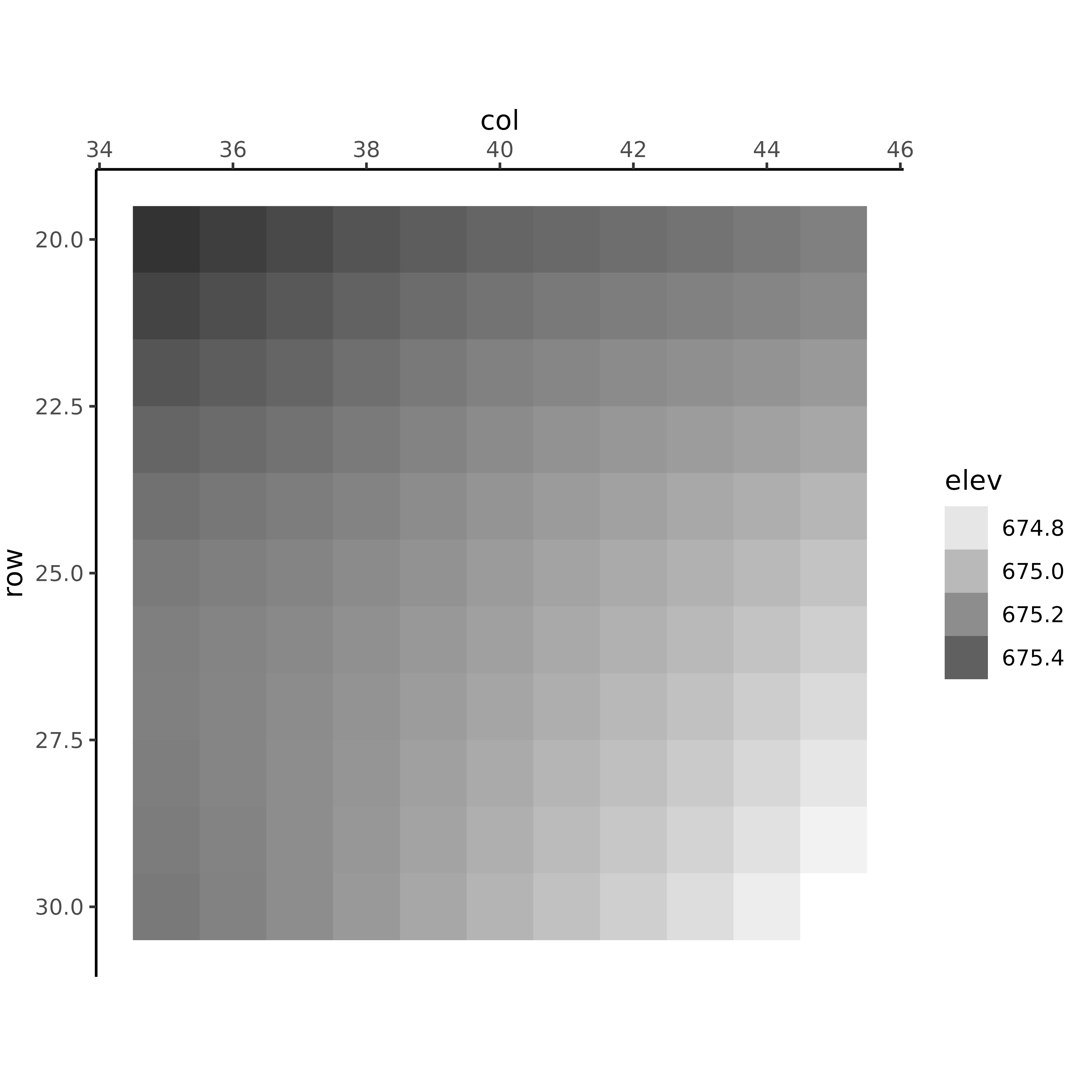

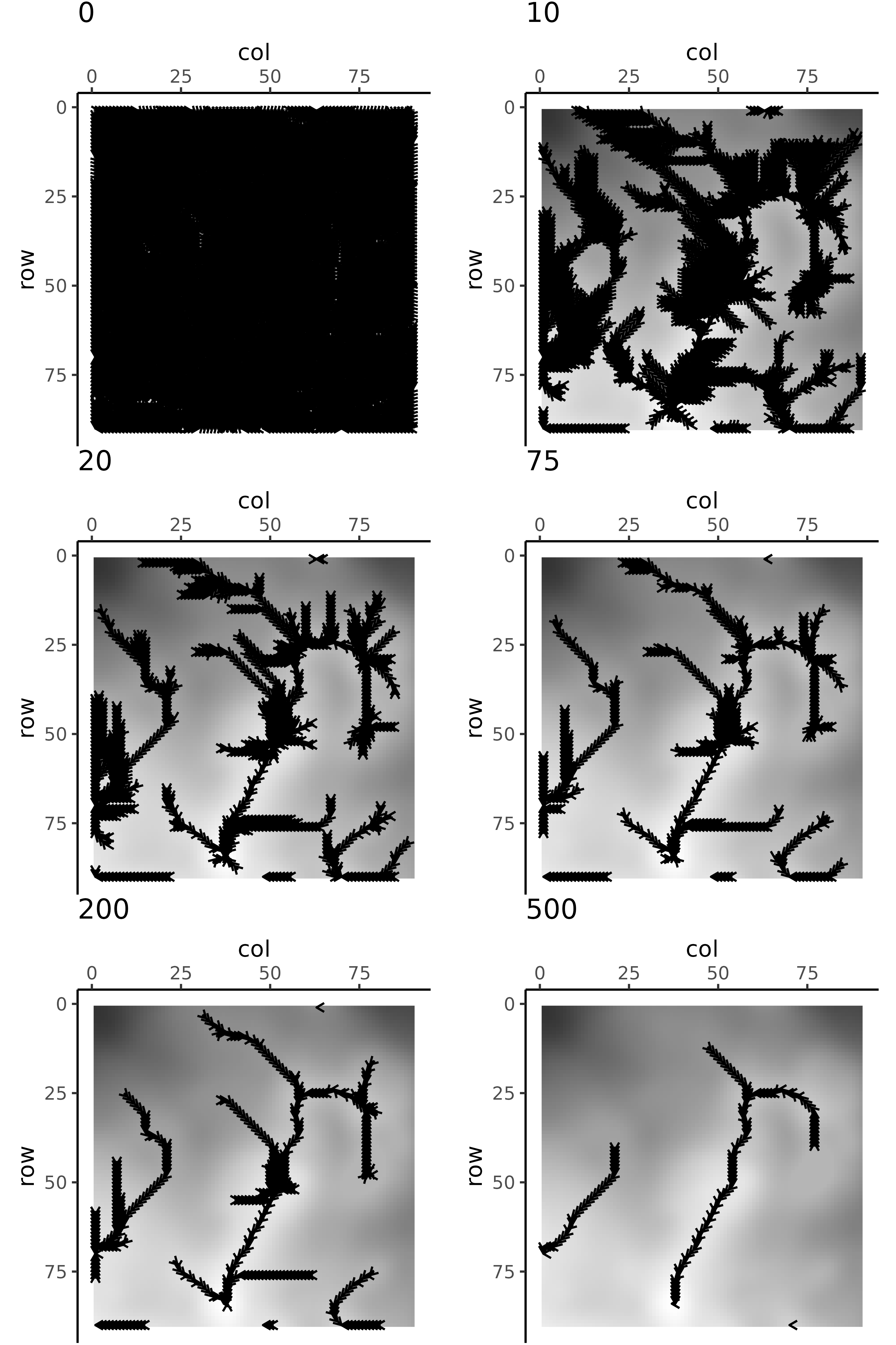
Flow directions by upslope area

You can filter the flow directions to show only those with an upslope area greater than some threshold:

flow_plot(dem, type = "elevation", dir = TRUE, upslope_threshold = 500)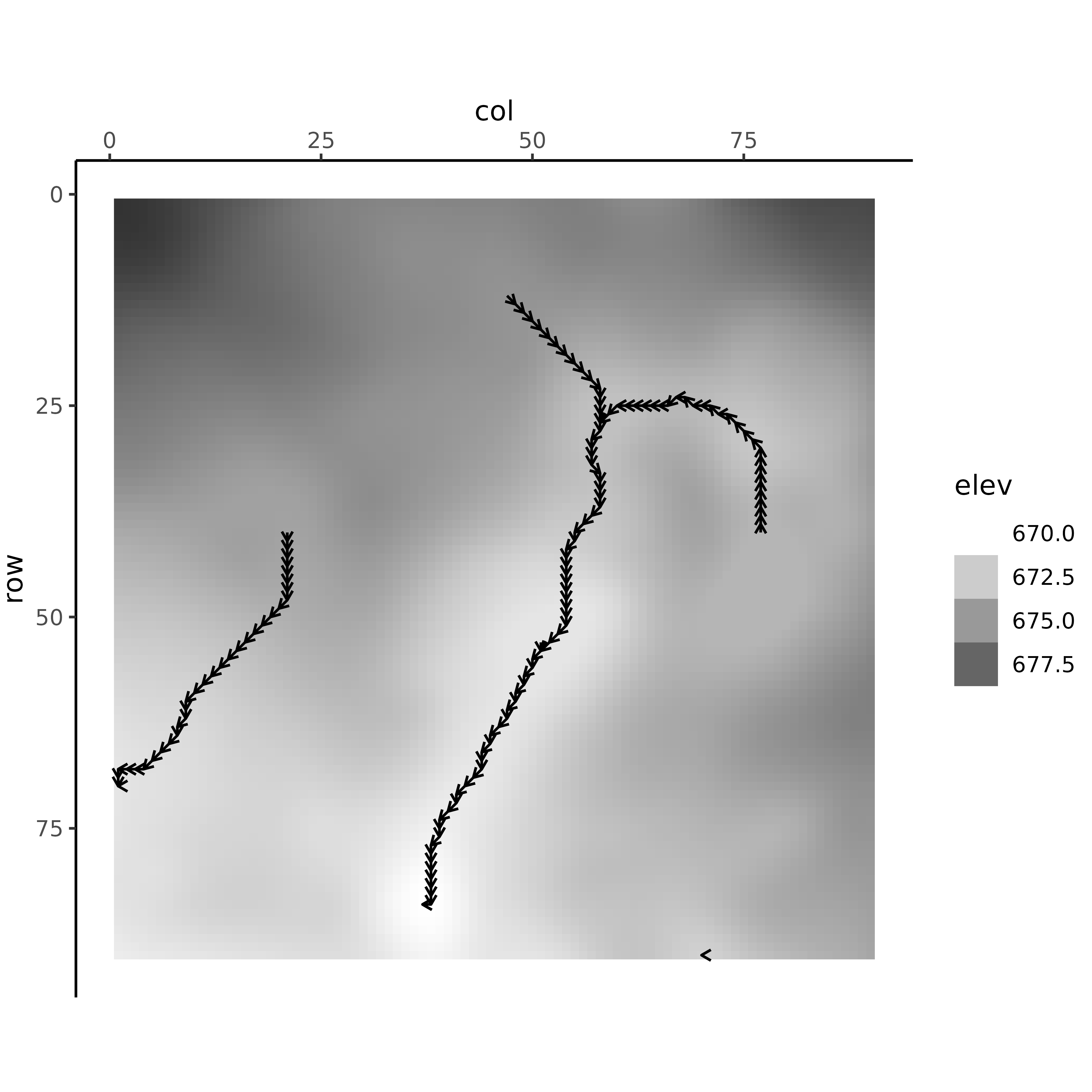

Comparing different upslope thresholds:

Ridge Lines

To look at ridge lines, use the inverted dem files

flow_plot(inverted_dem, type = "elevation", dir = TRUE, upslope_threshold = 250)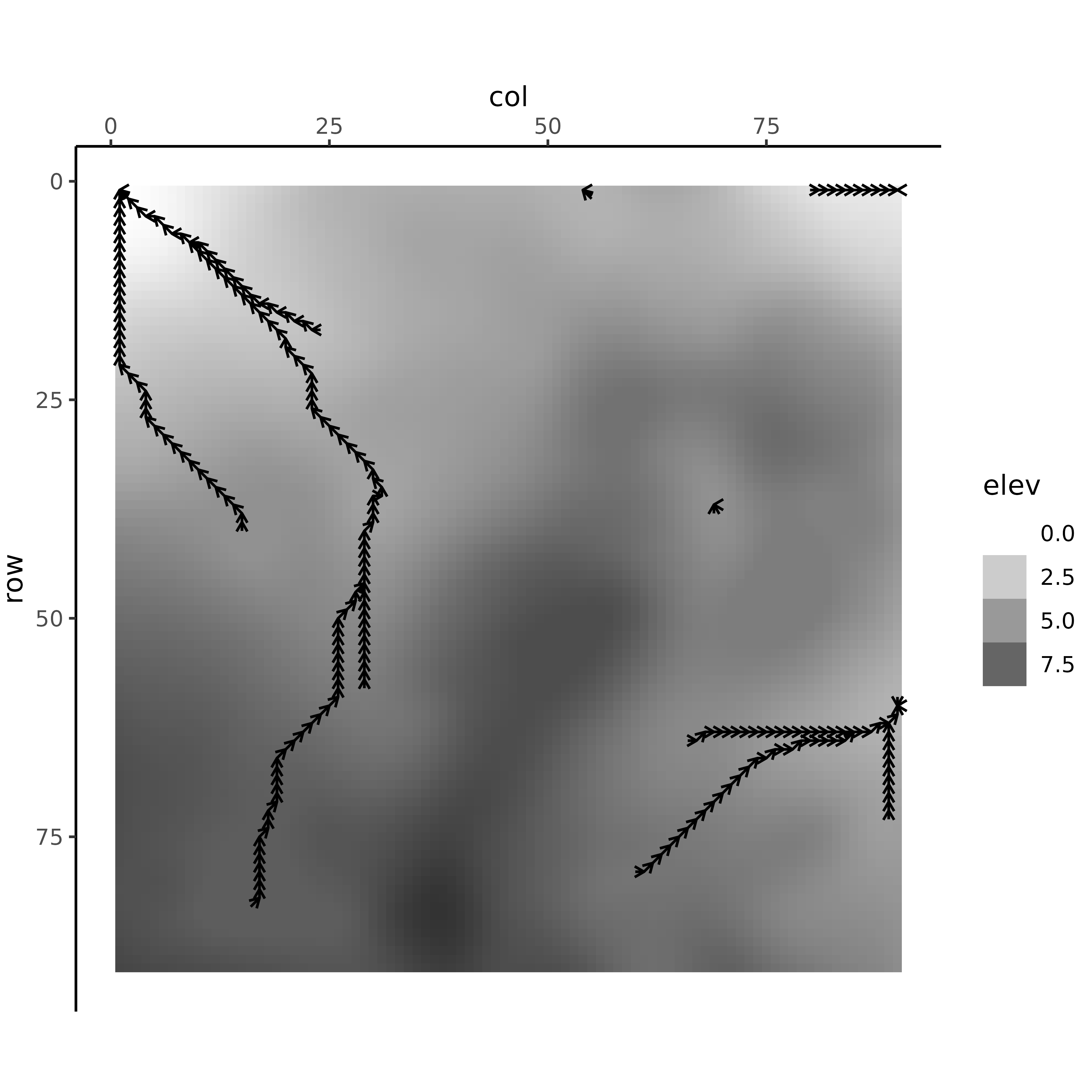

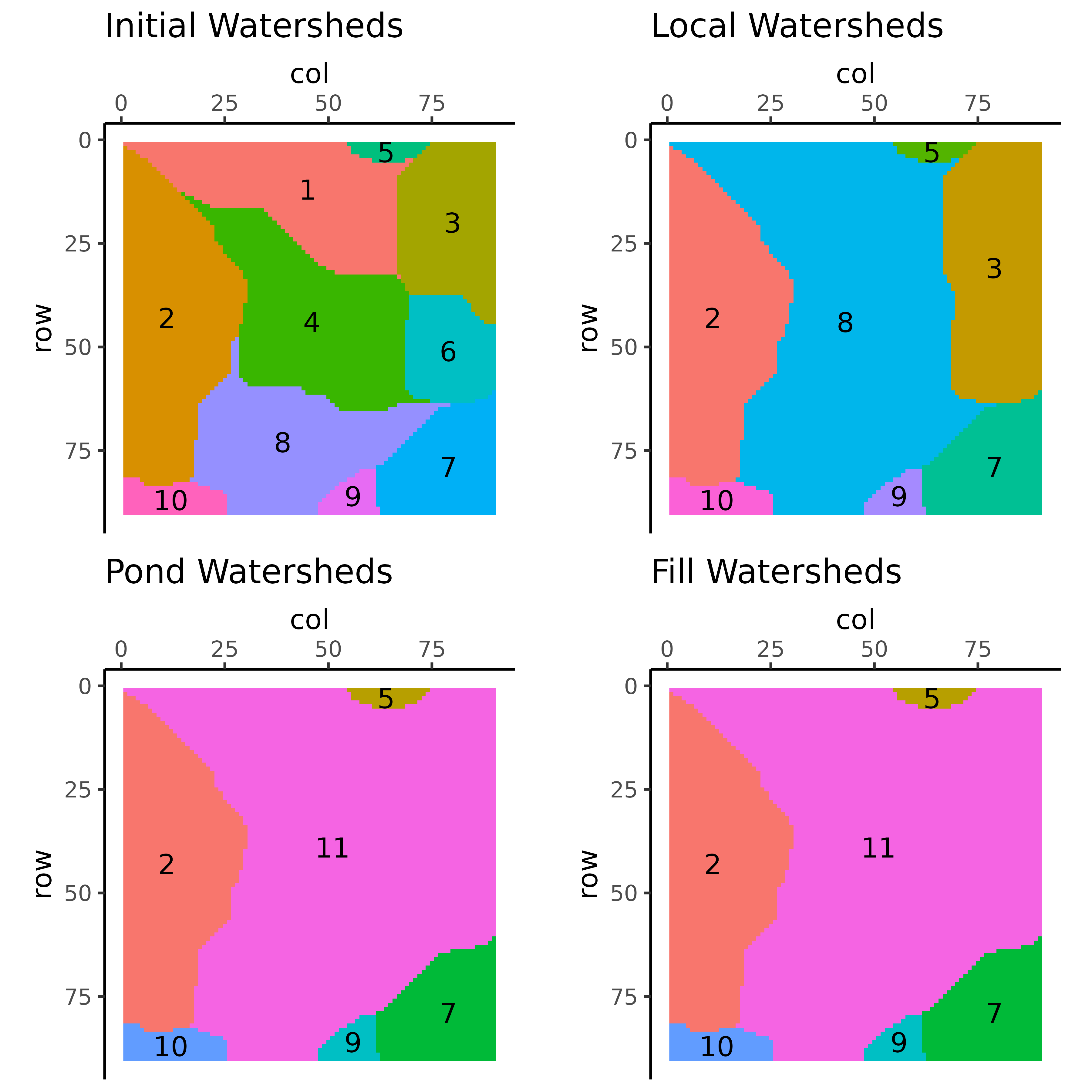
Watersheds

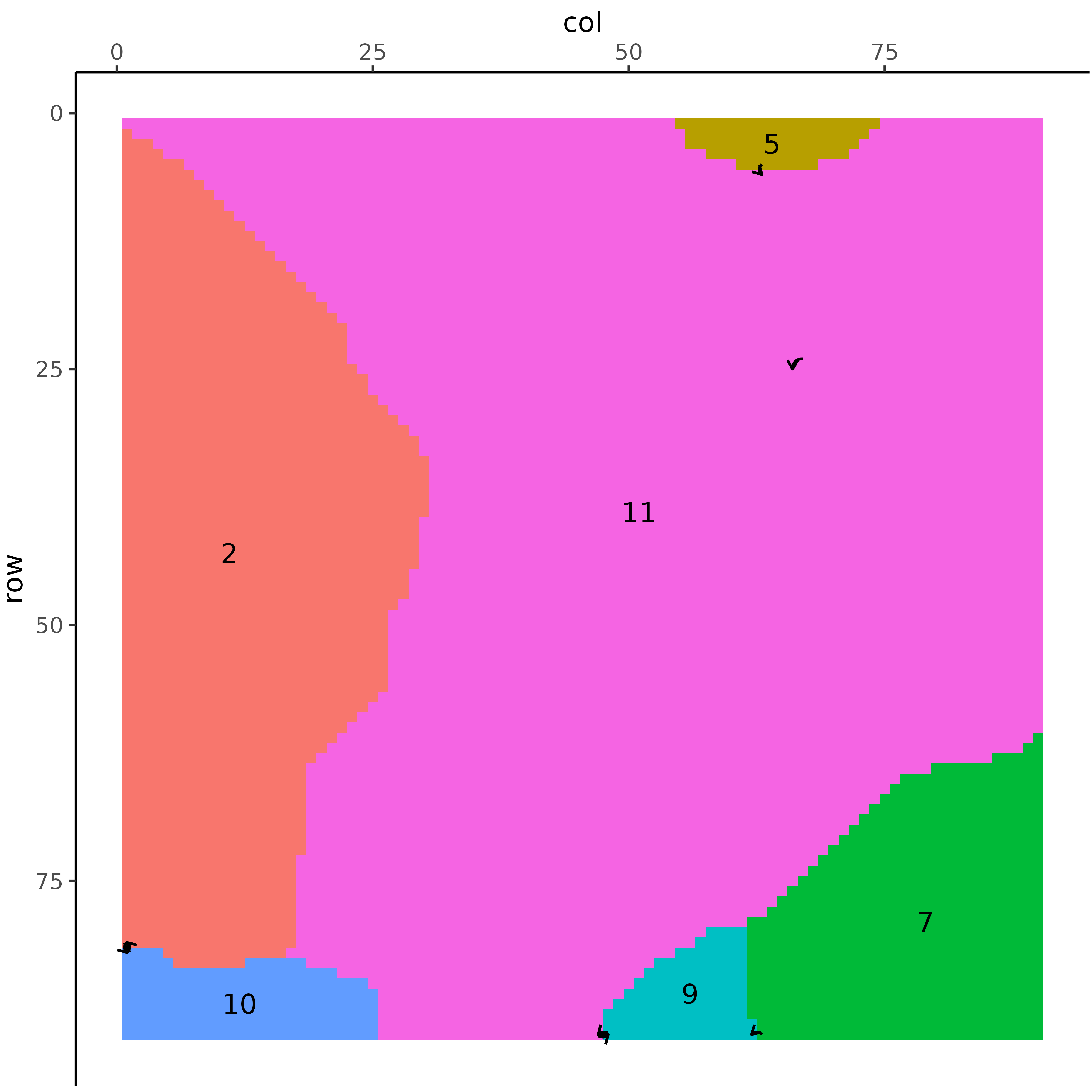
You can also highlight watersheds

flow_plot(db = dem, type = "elevation", shed = TRUE, shed_type = "initial") +
  labs(title = "Initial Watersheds")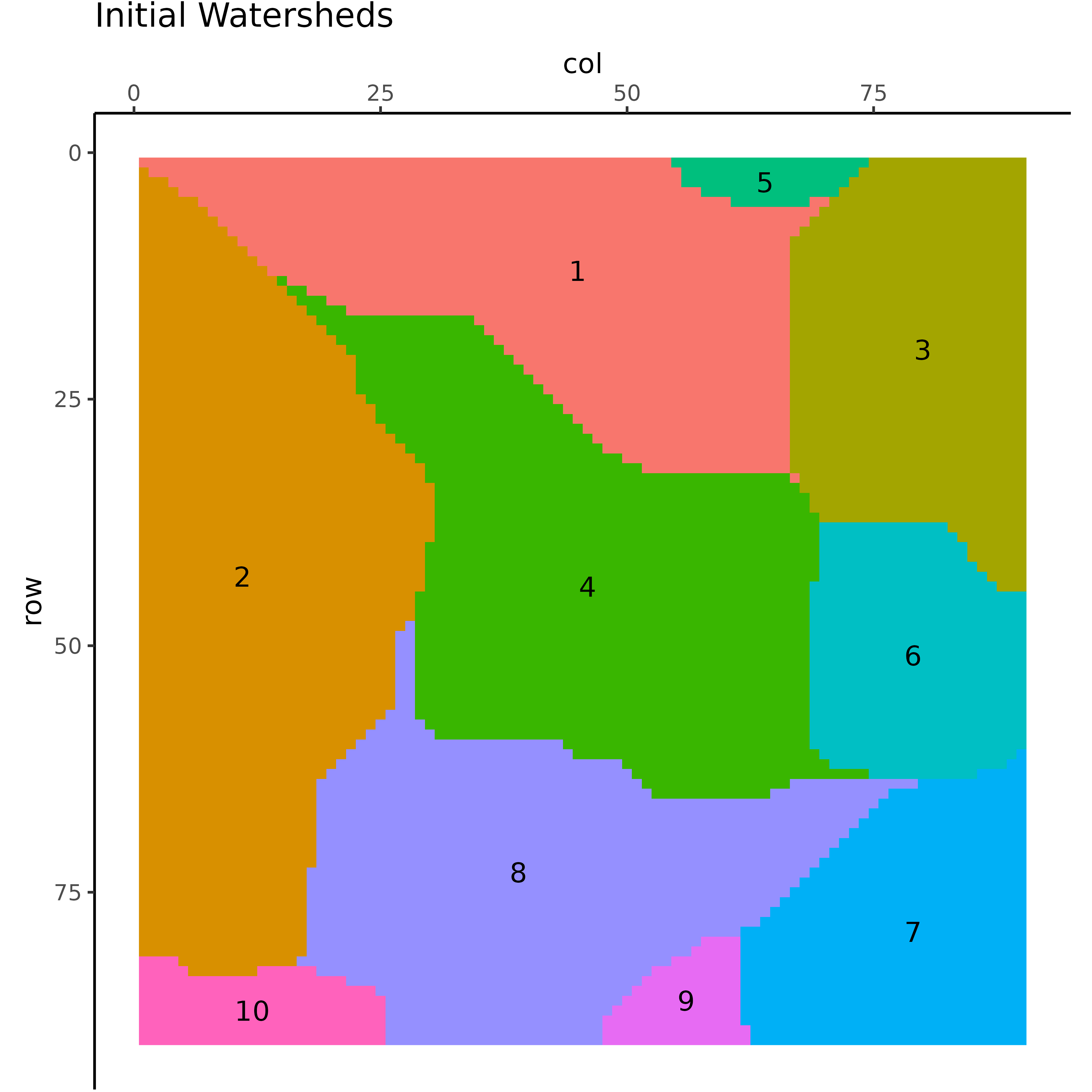

Watershed pits

flow_plot(db = dem, type = "elevation", shed = TRUE, shed_type = "initial", 
          pits = TRUE)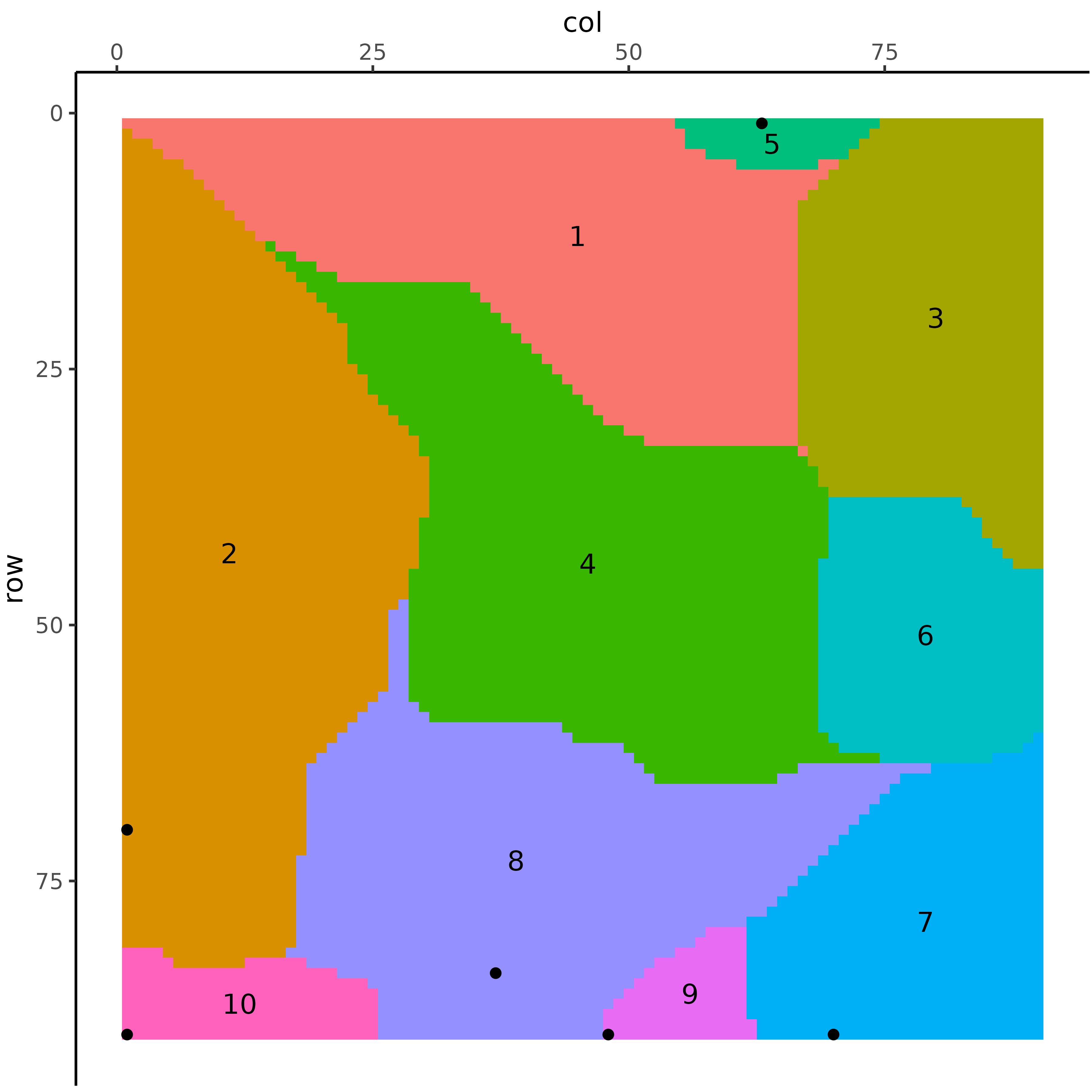

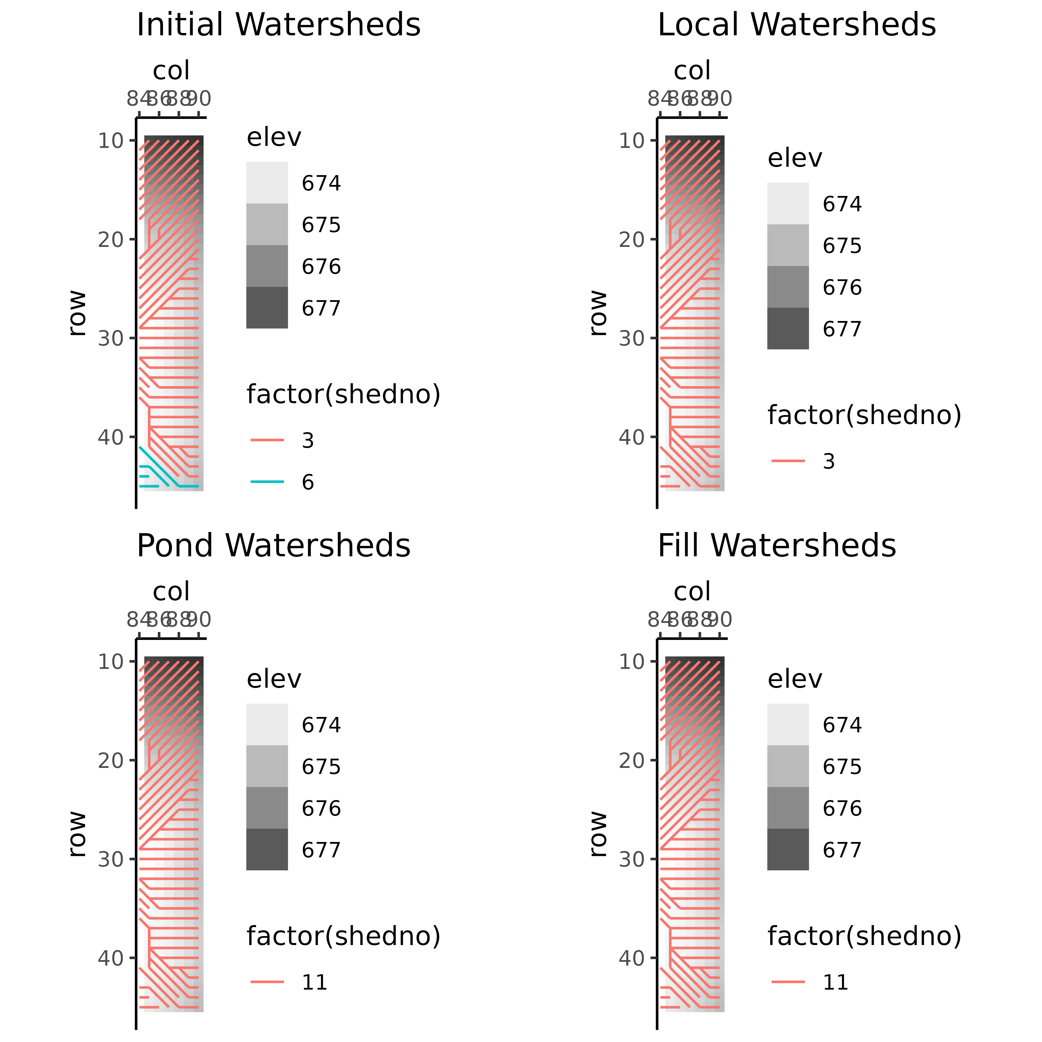
Comparing watersheds at different stages of pit removal

Initial = no removal
Local = smoothing, only small pits removed
Pond = looking at overflow in 2nd pit removal process
Fill = looking at overflow in a second way in 3rd pit removal process

Watersheds by flow paths

flow_plot(db = dem, type = "elevation", shed = TRUE, 
          shed_type = "initial", dir = TRUE)

Subsets still apply

flow_plot(db = dem, type = "elevation", shed = TRUE, 
          rlim = c(30,60), clim = c(45,75),
          shed_type = "initial", dir = TRUE)

Look at how watersheds combined in the upper right corner

Look at pour points

flow_plot(db = dem, type = "elevation", shed = TRUE, shed_type = "pond", 
          stats = pond_stats)

Take a closer look

flow_plot(db = dem, type = "elevation", shed = TRUE, shed_type = "pond",
          rlim = c(0, 40), clim = c(110, 150), stats = pond_stats)

Steffi LaZerte

2024-10-01